Previous - Measures Of Central Tendency

The mean, median and mode are useful; however, they are limited in that they do not say anything about the variation or dispersion of the actual data values compared with the mean, median and mode. A measure is needed and this measure is the variance or standard deviation. The following are two measures of variance.

Sample variance,  "$s^2 = \dfrac {\sum \left( X - \bar X \right) ^2}{n-1}  $"

Population variance, "$ \sigma^2 = \dfrac {\sum \left( X - \mu \right) ^ 2}{N} $"

where
"$ X $": individual data point
"$ \mu $" : mean of data points
"$ N $": total # of data points

The following are the measures of standard deviation:

Sample Standard Deviation, "$s = \sqrt {\dfrac {1}{N - 1} \underset{i=1}{\overset{N}{\sum}} \left( x_i - \bar x \right) ^2} $"

Population Standard Deviation, "$ \sigma = \sqrt {\dfrac {1}{N} \underset{i=1}{\overset{N}{\sum}} \left( x_i - \mu \right) ^2} $"

The above two equations are measures of the standard deviation which is the most common measure of variation. It is the square root of the variation. The value of the standard deviation tells us how closely the values of the data set are clustered around the mean. A lower standard deviation means that many of the values of the variables of the data set are clustered around the mean. On the other hand, a large standard deviation means that the values of the data set are far from the mean in many instances. Therefore, the actual values are different from the mean.

For example, if we have a data set as:

"$ 4, 5, 6, 7, 8, 4 \text{ and } 9 $"

The mean which is:

"$ \dfrac{\left(4+5+6+7+8+4+9 \right)}{7} = 6.14 \text{ or } 6 $"

"$ \begin{align} \text{Variance} & = \dfrac{ \left( 4 - 6 \right) ^2 + \left( 5 - 6 \right) ^2  + \left( 6 - 6 \right) ^2 + \left( 7 - 6 \right) ^2 + \left( 8 - 6 \right) ^2 + \left( 4 - 6 \right) ^2 + \left( 9 - 6 \right) ^2}{7} \\ & = \dfrac {4 + 1 + 0 + 1 + 4 + 4 + 9}{7} = \dfrac{23}{7} = 3.28 \end{align} $"

 So the variance is 3.28 about the mean of 6. The standard deviation is the square root of the variance which is

"$ \sigma ^2 = 1.81 $"

Interpreting the Standard Deviation

Larger values mean that the set of data is more spread out around the mean, while smaller values mean that the set of data is less spread out around the mean. If the data set has an approximately symmetrical and bell-shaped distribution (i.e. is approximately normally distributed), then we can say that:

• Roughly 68% of the data will lie within ONE standard deviation of the mean.
• Roughly 95% of the data will lie within TWO standard deviations of the mean.
• More than 99% of the data will lie within THREE standard deviations of the mean.

Effect of Distribution Shape on Measures of Central Tendency

It is interesting to consider the possible effect the shape of a distribution, that is, the shape of the curve might have on measures of central tendency. This consideration in turn might lead us to decide which measure of central tendency, the mean, the median, or the mode, is the best to use in a given situation.

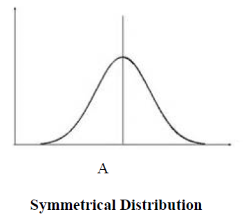
In a symmetrical distribution, the mean lies along the abscissa at the center of the curve. However, the median, with an equal number of scores above and below it also lies at the same point. The most frequently occurring score, the mode, also lies at this same point. Thus point A in the figure below represents the mean, the median, and the mode.

In general the mean is the best measure of central tendency. In its calculation, it does represent all of the scores. If any score changes, the mean will change. This is not true of the median or mode. This implies that extreme scores in either the high or the low direction will have a much greater effect on the mean than they would have on the median or the mode. For example, take the situation where we have a small factory with 9 employees and a manager. Each of the employees is paid $19,000 per year, while the manager is paid $29,000.

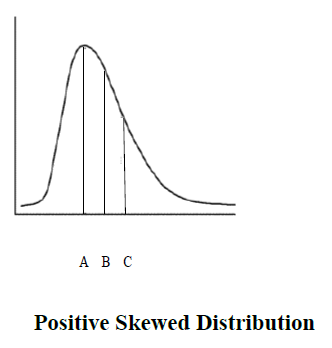
This frequency distribution is said to be positively skewed, that is the long slope of the curve is in the positive direction. A positively skewed distribution is caused by a relatively few high scores, or in the present example a single high score (the manager's salary). The total for salaries is $200,000 so the mean salary would be $20,000. We can see that the mean has been drastically increased relative to the mode and the median. In the figure below with a positively skewed distribution, the mode is the highest point of the curve and is represented by point A. The mean is the most shifted in the positive direction and is represented by point C. The median, in the typical situation of a positively skewed distribution, lies between the mode and the mean and is represented by point B. In this case of a skewed distribution, the median is probably a better measure of central tendency than the mean.

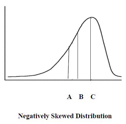
We can also have a skewed distribution because of a relatively few very low scores. For example, you live in a neighborhood in which there are nine homes valued at $150,000, $140,000, $160,000, $150,000, $160,000, $170,000, $160,000, $150,000, and $160,000. There is one small empty lot in the area and someone builds a very small garage on it with a valuation of $20,000. If we were to make a frequency polygon of these 10 values it would be a negatively skewed curve. The mode is $160,000, the median $155,000 (using the $20,000 as the first value) and the mean is $142,000. In the following distribution, point C represents the mode, point B represents the median, and point A represents the mean. This distribution, of course, represents a negatively skewed distribution. In this case, the median might be a better measure of central tendency than the mean.

Measurement of Skewness

Having discussed variance and deviation from the mean in relation to the normal curve, we now turn to the shape of the normal curve- skewness and kurtosis. You can get a general impression of skewness by drawing a histogram. Another way of testing for skewness is to know the shape of a curve – it should be normal. Many statistical inferences require that a distribution be normal or nearly normal. A normal distribution has skewness and excess kurtosis of 0. Therefore, if the distribution is close to those values then it is probably close to normal. Finally, skewness can be computed as follows:

The moment coefficient of skewness of a data set is as follows:

"$ g_1 = \dfrac {m_3}{m_2 ^ {3/2}} $" 

where

"$m_3 = \dfrac {\sum \left( X - \bar X \right) ^3}{n}  $" and "$m_2 = \dfrac {\sum \left( X - \bar X \right) ^2}{n}  $"

x̄ is the mean and n is the sample size. m3 is called the third moment of the data set. m2 is the variance, the square root of this is the standard deviation.

There is need to choose one of two different measures of standard deviation, depending on whether you have data for the whole population or just a sample. The same is true of skewness. If you have a sample from the population, then g1 above is the measure of skewness, however, skewness for the population is measured by the following equation:

"$ G_1 = \dfrac {\sqrt{n \left( n - 1 \right) }}{n - 2} g_1 $"

See the data in the following table for illustration where n = 85.

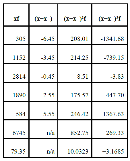
Using the above data, skewnes can be calculated as follows:

"$ g_1 = \dfrac {m_3}{m_2 ^ {3/2}} = \dfrac {-3.1685}{10.0323 ^ {3/2}} = -0.997 $"

This is the case for a sample from the population. The following is the case for the entire population:

"$ \begin{align} G_1 & = \dfrac {\sqrt{n \left( n - 1 \right) }}{n - 2} g_1 \\ & = \left[ \dfrac {\sqrt {\left( 85 \times 84 \right) }}{83} \right] \left[ \dfrac {-3.1685}{10.0323 ^ {3/2}} \right] = -0.1015 \end{align} $"

If skewness is positive, the data are positively skewed or skewed right, meaning that the right tail of the distribution is longer than the left. If skewness is negative, the data are negatively skewed or skewed left, meaning that the left tail is longer.

• If skewness = 0, the data are perfectly symmetrical.
• If skewness is less than −1 or greater than +1, the distribution is highly skewed.
• If skewness is between −1 and −½ or between +½ and +1, the distribution is moderately skewed.
• If skewness is between −½ and +½, the distribution is approximately symmetric.

With a skewness of −0.1015, the sample data are approximately symmetric.

Kurtosis

If a distribution is symmetric, the next question is about the central peak: is it high and sharp, or short and broad. The height and sharpness of the peak relative to the rest of the data are measured by a number called kurtosis. Higher values indicate a higher, sharper peak; lower values indicate a lower, less distinct peak. Higher kurtosis means more of the variability is due to a few extreme differences from the mean, rather than a lot of modest differences from the mean.

• A normal distribution has kurtosis exactly 3 (excess kurtosis exactly 0). Any distribution with kurtosis ≈3 (excess ≈0) is called mesokurtic.
• A distribution with kurtosis <3 (excess kurtosis <0) is called platykurtic. Compared to a normal distribution, its central peak is lower and broader, and its tails are shorter and thinner.
• A distribution with kurtosis >3 (excess kurtosis >0) is called leptokurtic. Compared to a normal distribution, its central peak is higher and sharper, and its tails are longer and fatter.

Next - Discrete Random Variables And Their Probability Distribution