Previous - Sampling

Hypothesis Testing

In statistics, a hypothesis is a statement about a property of a population. There are four (4) main steps in hypothesis testing. They are:

1. Specification of the null and alternative hypothesis: The null hypothesis is a hypothesis about a population parameter. The purpose of hypothesis testing is to test the viability of the null hypothesis in the light of sample data. The null hypothesis either will or will not be rejected as a viable possibility.

   The null hypothesis is a statement about the population statistic while the alternate hypothesis is a claim to be tested. There are three ways to set up a null and alternate hypothesis.

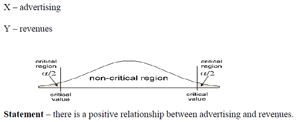
   1. Equal hypothesis verses not equal hypothesis (two-tailed test)

      H₀ : μ = 0 there is no relationship between advertising and revenues.

      H₁ : μ ≠ 0 there is a very strong relationship between advertising and revenues.

      

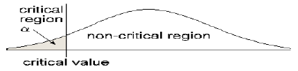
   2. Equal hypothesis verses less than hypothesis (left-tailed test)

      H₀ : μ = 0

      H₁ : μ < some value

      

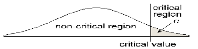
   3. Equal hypothesis verses greater than hypothesis (right-tailed test)

      H₀ : μ = 0

      H₁ : μ > some value

      

2. Setting the Significance Level: Suppose 90 different samples were taken from the same population. The value or mean for each of these will not be the same. Which of these 90 samples should be used as the estimate for the population mean? The answer is any sample mean and there is no way to guarantee that the sample that we choose is the best one. However, the best way is to assume that it falls between an interval so we will need to create one for each sample, so that the population mean, will be contained in approximately 95% or 90% or 99% whichever is chosen of those intervals. The 95% is called the degree of confidence. The Greek letter alpha, "$ \alpha $", is used to represent a probability or area. The significance level,, is the same as in the degree of confidence. The degree of confidence is the probability "$ \left( 1 - \alpha \right) $" that is described above.

   In hypothesis testing, the significance level is the criterion used for rejecting the null hypothesis. The critical region is the region under the normal curve that causes a rejection of the null hypothesis. This region can be left-tailed, right-tailed or two-tailed.

   Decision Rule:

   1. Reject H₀ if test statistic < c.v. (left) or test statistic > c.v. (right);
   2. Reject H₀ if the test statistic falls in the critical region;
   3. Reject H₀ if the test statistic is more extreme than the critical value.

3. The third step is to calculate a test statistic which can be determined by the following:

   "$ \bbox[30px,border:2px solid black] {Z=\dfrac{\bar x - \mu}{\sigma / \sqrt{n}}}$"

4. The fourth step is to compare the t-statistic with the critical values. If the calculated t statistic is greater than the critical value, we will reject the null hypothesis and accept the alternative hypothesis (See the following example).

Example:

Suppose 150 college students were asked their Intelligence Quotient (IQ). From the data you find out that x=120 and σ=11.3. A college professor says that he knows the population mean, μ is less than 116. Using a 0.05 significance level, determine if the professor may be correct.

Solution: The people running the project want the professor to be wrong, so you want to prove the claim "The population mean is greater than 116." (Remember that only the alternate hypothesis can be supported, so the statement should NOT contain equality.) So in this case let:

H₀ : μ = 116

H₁ : μ > 116

With the null hypothesis H₀: μ= 116, the critical region is in the right tail. With a right-tail area of 0.05 the critical value is z=1.645. The critical value is used to set up the critical region. With n=150, σ=11.3, x=120 and μ= 116, the test statistic is 4.34. This value is right of the critical value of 1.645. Hence, the test statistic is in the critical region, which means that the null hypothesis is rejected. Since the null hypothesis is rejected, the alternate hypothesis is supported. Thus, the population mean is greater than 116. The professor is wrong.

Example:

TSTT provides long distance telephone services. Based on the company’s records, the average length of all calls in 2010 was 12.44 minutes. TSTT wants to determine whether the mean length of currents calls is different from 12.44 minutes. A sample of 150 such calls during the year produced a mean length call of 13.71 minutes. The standard deviation of call is 2.65 minutes. Using a 2% significance level, can you conclude that the mean of all current long distance calls is different from 12.44 minutes?

Step 1: Setting the Hypotheses

H₀ : μ = 12.44

H₁ : μ ≠ 12.44

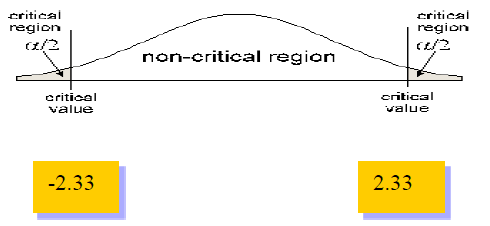
Step 2: Setting the Confidence Level & Determining the Rejection Region

The significance level in this case is: 2 % or .02. This is a two-tail test because of the not equal sign and so we divide .02 by 2 to get: .01. When we look at the .01 in the t table for 150 or ∞, we get 2.33 and -2.33.

Step 3: Calculate a test statistic which can be determined by the following:

"$ Z = \dfrac{\bar x - \mu}{\sigma / \sqrt{n}} $"

"$ Z = \left( 13.71-12.44 \right) / .21637 = 5.87 $"

Because "$ \sigma = 2.65 / \left( 150 \right)^\frac{1}{2} = .21637 $"

Step 4: The fourth step is to compare the t-statistic with the critical values.

Because 5.87 is greater than 2.33 and it falls in the rejection region, we can reject the null hypothesis that the mean telephone calls is 12.44. Therefore, the mean telephone call today is different from 12.44 minutes.

The above examples are from the critical-value approach which is called the classical approach to hypothesis testing. In this approach, the test statistic is compared with the critical value. One problem with the Classical Approach is that if a different level of significance is desired, a different critical value must be read from the table.

Another approach to hypothesis testing is that of the p-value approach which is short for Probability Value; this approaches hypothesis testing from a different manner. Instead of comparing z-scores or t-scores as in the classical approach, we are comparing probabilities, or areas. The level of significance (alpha) is the area in the critical region. That is, the area in the tails to the right or left of the critical values.

The p-value is the area to the right or left of the test statistic. If it is a two tail test, then look up the probability in one tail and double it. If the test statistic is in the critical region, then the p-value will be less than the level of significance. It does not matter whether it is a left tail, right tail, or two tail test. This rule always holds. Reject the null hypothesis if the p-value is less than the level of significance. You will fail to reject the null hypothesis if the p-value is greater than or equal to the level of significance. If the t-statistic is in the critical region, the null hypothesis is rejected and the alternative is accepted. In this case, the p-value will be less than the level of significance.

Example:

At a manufacturing company, it takes 90 minutes for new workers to learn a job. Recently new technology was installed and the company wants to see if this will result in the mean time being different from 90 minutes. A sample of 20 workers revealed that it took on average of 85 minutes for them to learn the new job with the new technology. All the learning times for the workers are assumed to be normally distributed with a standard deviation of 7 minutes. Find the p-value for the test that the mean learning time for the job with the new technology is different from 90 minutes. What will your conclusion be if "$ \alpha = .01 $".

Step 1: Setting the Hypothesis:

H₀ : μ = 90 minutes

H₁ : μ ≠ 90 minutes

Step 2: Setting the Confidence Level & Determining the Rejection Region:

"$ \alpha = .01 $"

"$ Z = \left( 85-90 \right) / 1.5652 = -3.19 $"

Because "$ \sigma = 7 / \left( 20 \right)^\frac{1}{2} = 1.5652 $"

Step 3: Calculate a test statistic which can be determined by the following:

When we look at the z table for -3.19, we get .0007.

Consequently, because we need to double this .0007, the p-value = 2(.0007) = .0014.

Step 4: The fourth step is to compare the p-value with the significance level and make the decision:

When we compare .0014 to .01, we see that the statistic is smaller than the .01 so we can reject the null hypothesis. Therefore, the mean time taken to complete the job function is different from 90 minutes.

As a rule of thumb:

The test statistic is to the p-value as the critical value is to the level of significance.

There are several ways to refer to the significance level of a test, and it is important to be familiar with them. All of the following statements, for example, are equivalent:

• The finding is significant at the .05 level.
• The confidence level is 95 percent.
• The Type I error rate is .05.
• The alpha level is .05.
• α = .05.
• There is a 95 percent certainty that the result is not due to chance.
• There is a 1 in 20 chance of obtaining this result.
• The area of the region of rejection is .05.
• The p-value is .05.
• p = .05.

The Z – table gives you the area under the curve while the t table gives you the critical value. In arriving at the critical value, we need to calculate the number of degrees of freedom by n – 1.

Two main types of error can occur:

1. Type I error (also, α error, or false positive) - the error of rejecting a null hypothesis that should have been accepted and;
2. Type II error (β error, or a false negative) - (β) the error of accepting a null hypothesis that should have been rejected.

Next - Regression Basics