Previous - Difference between Z Distribution and T Distribution
Confidence Intervals/Limits
Confidence Intervals/Limits are a way of taking data from a sample and saying something about the population from which the sample was drawn. Interval estimates are often desirable because the estimate of the mean varies from sample to sample. Instead of a single estimate for the mean, a confidence interval generates a lower and upper limit for the mean. The interval estimate gives an indication of how much uncertainty there is in our estimate of the true mean. The narrower the interval, the more precise is our estimate.
Confidence limits are expressed in terms of a confidence coefficient. Although the choice of confidence coefficient is somewhat arbitrary, in practice 90%, 95%, and 99% intervals are often used, with 95% being the most commonly used. As a technical note, a 95% confidence interval does not mean that there is a 95% probability that the interval contains the true mean. The interval computed from a given sample either contains the true mean or it does not. Instead, the level of confidence is associated with the method of calculating the interval. The confidence coefficient is simply the proportion of samples of a given size that may be expected to contain the true mean. That is, for a 95% confidence interval, if many samples are collected and the confidence interval computed, in the long run about 95% of these intervals would contain the true mean.
We can express the confidence coefficient is as a multiplier and this multiplier is chosen depending on the confidence you want to place in your interval: do you want to be 99 percent sure you are right? 95 percent? Or are you satisfied with 67 percent? Note that higher confidence percentages come at the price of making the interval wider and therefore any forecast less precise.
RULE OF THUMB:
- use a multiplier of 1.0 for about 67 percent confidence,
- a multiplier of 2.0 for about 95 percent confidence,
- a multiplier of 3.0 for about 99 percent confidence
The following table can be used to approximate the multiplier for estimation of the confidence interval.
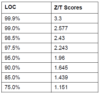
However, it is better to use the statistic in the t-table in the Appendix.
Example:
Given the following information: standard deviation of population = 100, sample mean = 600, sample size = 20. Construct an approximate 67 percent and 95 percent confidence interval for the mean.
Solution:
We need to find the variance of the sample mean = variance of population / N = 10,000 / 20 = 500. The variance of the population which is 10,000 was derived by multiplying the standard deviation of 100 by itself. This is so because the standard deviation is the square root of the variance. If the square root of the variance which is the standard deviation is 100, then the variance will be 100 times 100 which is 10,000. Therefore, the standard errors of the sample mean is the square root of 10,000/20 which is 22.3. Expressed alternatively will be 100/4.472 = 22.36.
For a 67 percent confidence interval, the multiplier is 1. Hence the 67 percent confidence interval = 600 +/- (1) 22.36 = 577.64 to 622.36.
For a 95 percent confidence interval, the multiplier is 2. Hence the 95 percent confidence interval will be 600 +/- (2) 22.36 = 555.28 to 644.22.
Note that the higher confidence level required a wider interval estimate for the mean.
Example:
Suppose that we conducted a survey of 19 millionaires to find out what percent of their income the average millionaire donates to charity. We discover that the mean percent is 15 with a standard deviation of 5 percent. Find a 95% confidence interval for the mean percent. Assume that the distribution of all charity percents is approximately normal.
Solution
We use the formula:
"$ \begin{align} \bar x \pm Z \ast \dfrac{s}{\sqrt n} &&& \bar x - \dfrac{ts}{\sqrt n} \text{ to } \bar x + \dfrac{ts}{\sqrt n} \end{align} $"
(Notice the t instead of the z and s instead of σ)
We get
"$ 15 + t_c 5 / \sqrt{19} $"
Since n = 19, there are 18 degrees of freedom. Using the table in the back of the book, we have that
"$ t_c = 2.10 $"
Hence the margin of error is
"$ 15 \pm 2.00 \left( 5 \right) / \sqrt{19} = \pm 2.4 $"
We can conclude with 95% confidence that the millionaires donate between 12.7% and 17.3% of their income to charity.
Example
Suppose that we check for clarity in 50 locations in Lake Asphalt and discover that the average depth of clarity of the lake is 14 feet. Suppose that we know that the standard deviation for the entire lake's depth is 2 feet. What can we conclude about the average clarity of the lake with a 95% confidence level?
Solution
"$ \begin{align} \bar x \pm Z \ast \dfrac{s}{\sqrt n} &&& \bar x - \dfrac{ts}{\sqrt n} \text{ to } \bar x + \dfrac{ts}{\sqrt n} \end{align} $"
"$ \begin{align} &= 14 \pm \left( 1.95 \right) 2/ \sqrt{50} \\ &= 14 \pm \left( 2.00 \right) 2 / \left( 7.071 \right) \\ &= 14 \pm \left( 2.00 \right) .2828 \\ &= 14 \pm 0.56 \left( \text{this is the margin of error} \right) \\ &= \left( 13.44 \text{ to } 14.56 \right) \end{align} $"
Proportions
Suppose we need to find the proportion of individuals in a population who possess a certain attribute. For instance, for planning purposes we may require to know:
- The proportion of defective items coming off a production line in a shift;
- The proportion of pensioners in a country;
- The proportion of householders in a major city who wish to possess cable television.
Provided the proportion is not expected to be very small, we can use the same technique to find this information as we used for measurements of continuous variables. The results of a sample survey are used to estimate the population proportion. For the population:
"$ \text{Let p } = \dfrac{\text{ Number of individuals possessing the attribute}}{N} $"
"$ \text{Let q } = \dfrac{\text{ Number of individuals not possessing the attribute}}{N} $"
where N is the population size.
For the sample:
"$ \text{Let p } = \dfrac{\text{ Number of individuals possessing the attribute}}{n} $"
"$ \text{Let q } = \dfrac{\text{ Number of individuals not possessing the attribute}}{n} $"
and p + q = 1
Then p is the estimate of p and, by the Central Limit Theorem, p is normally distributed, so:
- A confidence interval for "$ \pi = p \pm z \left( \text{SE of p} \right) $" where z is the value of the standard normal of the chosen percentage and;
- The standard error of p can be shown to be "$ \sqrt{\dfrac{pq}{n}} $" which is estimated by "$ \sqrt{\dfrac{pq}{n}} $"
Example:
In a sample of 200 voters, 80 were in favour of reintroducing an incentive plan. Find a 95% confidence interval for the proportion of all voters who are in favour of this measure.
"$ p = 80/200 = 0.4 $"
"$ q = 1– p = 0.6, $"
"$ \begin{align} \text{SE of p} & = \sqrt{\dfrac{pq}{n}} \\ & = \sqrt{\dfrac{\left( 0.4 \right) \left( 0.6 \right)}{200}} \end{align} $"
Thus, a 95% confidence interval for "$ p = p \pm 1.96 \sqrt{\dfrac{pq}{n}} $"
"$ \begin{align} & = 0.4 \pm 1.96 \times 0.0346 \\ & = 0.4 \pm 0.0679 \\ & = 0.332 \text{ to } 0.468 \end{align} $"
Therefore, the proportion of voters in favour lies between 33% and 47%.