Previous - Hypothesis Testing

Regression Analysis

Regression is a statistical measure used to determine the strength of the relationship between one dependent variable (usually denoted by Y) and a series of other changing variables (known as independent variables). The two basic types of regression are linear regression and multiple linear regression, although there are non-linear regression methods for more complicated data and analysis. Linear regression uses one independent variable to explain or predict the outcome of the dependent variable Y, while multiple regression uses two or more independent variables to predict the outcome.

Regression analysis involves:

• The selection of the best fit or line when the data that are graphed do not lie on the line – this line will be the one that results in the least squared errors thus the name ordinary least squares;
• Estimation of a dependent variable (Y) based on values of an independent variable (X);
• Testing the relationship between two variables – using the explanatory or independent variable to predict the dependent variable and;
• Forecasting of some specified variables.

GRAPHICAL INTERPRETATION

The best way to understand the relationship between two variables is to graph the data with the independent variable being on the horizontal axis while the dependent variable being on the vertical axis.

For example, a company finds that its sales volume is dependent upon its advertising outlay. Advertising expenditures are budgeted to be $6 million next year. The following table states this relationship.

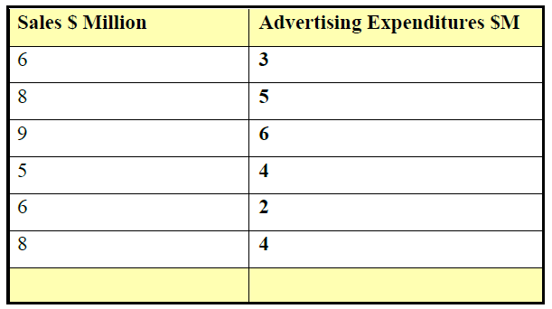
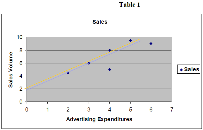
It can be noticed that all of the points plotted do not lie on the line. The fact that all data points are not on the line means that advertising expenditures are not the only predictor or estimator of sales volume for this company. There may be other important variables. There may also be errors involved in forecasting sales volume through advertising sales. Therefore there can be a number of possible lines that can be drawn. The idea is to choose the best of these lines; this is what regression analysis does.

LINEAR REGRESSION

In the regression model one of the assumptions is that there exists a relationship between the variables in the model. The simple or general regression model is as follows:

Y = β₀ + β₁ X + Є

where:

Y = dependent variable to be tested;
X – independent variable that will be used to make inferences on Y;
β₀ - the intercept that cuts the vertical axis;
β₁ – the coefficient to be estimated or the slope of the line;
Є – the error term or variance that estimates the residual or disparity.

Both the intercept and the coefficient are not known and must be estimated; the computer output gives estimates for these variables. They can also be calculated manually (which we will see later). The objective is to forecast or estimate Y and the difference between actual values and predicted or expected value is the error term. The errors can be either positive or negative and so we need to square the errors to eliminate any negative signs.

Because there can be a number of lines that can be drawn through the data points on the graph, we will need to choose the line that gives the least or smallest error and this is why regression analysis is sometimes called ordinary least squares (squaring the errors). There are formulas that can be used to obtain the equation of a straight line that would minimize the sum of the squared errors.

"$ \begin{align} X' & = \sum X/n \\ Y' & = \sum Y/n \\ \beta_1 & = \sum \left( X - X' \right) \left( Y - Y' \right) / \sum \left( X - X' \right)^2 \\ \beta_0 & = Y' - \beta_1 X' \end{align} $"

ASSUMPTIONS OF THE REGRESSION MODEL (this is elaborated in the Appendix)

Normal Distribution – the data must be distributed which means that it must be continuous and distributed around the mean; if we plot the data as a histogram it will be seen that the actual data deviates (both positive and negative) from the mean; the majority of the data points will be near the centre or mean of the graph;

Linearity – there is a straight line relationship between X and Y, the independent and dependent variables; if the equation is not linear it can be transformed by natural logarithms;

Homoscedasticity – the variance, error term or residual must be the same for all forecasted dependent variables year after year or for each year. Another way of saying this is that the variability in the independent variable is the same for all values of the dependent variable year after year; the variance must therefore be constant;

Multicolinearity – is where there is correlation among the explanatory or independent variables; because calculation of the regression coefficient is done through matrix inversion, there should be no correlation between the independent variables.

INTERPRETATION OF THE REGRESSION RESULTS

The following gives an overview of the key indicators used in assessing a regression output.

This R² is one of the main statistics that we will need to view from the regression output. It is called the coefficient of determination. The coefficient of determination, R squared, is used in linear regression theory as a measure of how well the regression equation fits the data. It is the square of R, the correlation coefficient, that provides us with the degree of correlation between the dependent variable, Y, and the independent variable X.

R² ranges from -1 to +1. If R² equals +1, then Y is perfectly proportional to X, if the value of X increases by a certain degree, then the value of Y increases by the same degree. If R² equals -1, then there is a perfect negative correlation between Y and X. If X increases, then Y will decrease by the same proportion. On the other hand if R=0, then there is no linear relationship between X and Y. R² varies from 0 to 1. This gives us an idea of how well our regression equation fits the data.

If R² squared equals 1, then our best fit line passes through all the points in the data, and all of the variation in the observed values of Y are explained by its relationship with the values of X. For example if R² is .80, then 80% of the variation in the values of Y is explained by its linear relationship with the observed values of X.

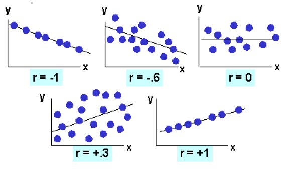
Another important statistic that will be on the computer output for the regression is that of the correlation coefficient and is symbolized as r which is the square root of r². r can assume values from -1 to + 1. It is negative if the slope of the line is downward sloping and positive if the slope of the regression line is upward sloping. If there is no relationship between the predicted values and the actual values the correlation coefficient is 0 or very low (the predicted values are no better than random numbers). As the strength of the relationship between the predicted values and actual values increases so does the correlation coefficient. A perfect fit gives a coefficient of 1.0. Thus, the higher the correlation coefficient the better.

The correlation coefficient is calculated as:

"$ p_{xy} = \dfrac{Cou \left( X,Y \right)}{\sigma_x \sigma_y} $"

The r can be visually represented by the following scattered plots:

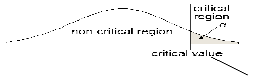
Another very important statistic is that of the actual t-statistic on the regression output. This depends on the level of significance used. The t-statistic is the coefficient divided by the standard error. That can be tested against a t distribution to determine how probable it is that the true value of the coefficient is really zero. This can be done be doing a hypothesis test where we attempt to reject the null hypothesis of there being no relation between the dependent and independent variables in favour of the alternative hypothesis of there being a relationship between the dependent and independent variables. This will require that we obtain the critical value (we will need the level of significance which could be 5% and the degree of freedom) to obtain this from the t distribution table and compare this with the calculated t statistic. If the t statistic is greater than the critical value, we will reject the null hypothesis in favour of the alternative hypothesis.

F Statistic or Test

In a multiple regression, a case of more than one x variable, we conduct a statistical test about the overall model. The basic idea is do all the x variables as a package has a relationship with the y variable? The null hypothesis is that there is no relationship and we write this in a shorthand notation as:

H_o: B₁ = B₂ = … = 0. If this null hypothesis is true the equation for the line would mean the x’s do not have an influence on y. The alternative hypothesis is that at least one of the beta’s is not zero. Rejecting the null means that the x’s as a group is related to y.

In practice we pick a level of significance and use a critical F to define the difference between accepting the null and rejecting the null.

To pick the critical F there are two types of degrees of freedom to be concerned about: there is the numerator and the denominator degrees of freedom to calculate. They are called this because the F statistic is a fraction. Numerator degrees of freedom = number of x’s, in general called p while the Denominator degrees of freedom = n – p – 1, where n is the sample size. As an example, if n = 10 and p = 2 we would say the degrees of freedom are 2 and 7 where we start with the numerator value. The critical F is 4.74 when alpha is .05.

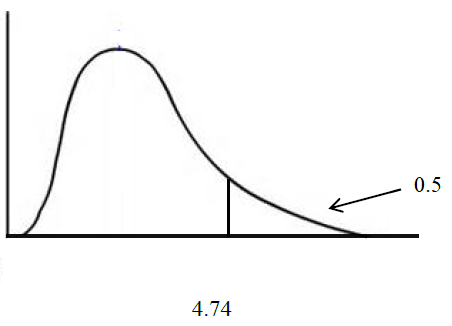
In our example here the critical F is 4.74. If the F statistic is 20.00, then this is greater than 4.74 and we would reject the null and conclude the x’s as a package have a relationship with the variable y.

P-value

The p-value is the area to the right or left of the test statistic. If it is a two tail test, then look up the probability in one tail and double it. If the test statistic is in the critical region, then the p-value will be less than the level of significance. It does not matter whether it is a left tail, right tail, or two tail test. This rule always holds. Reject the null hypothesis if the p-value is less than the level of significance. You will fail to reject the null hypothesis if the p-value is greater than or equal to the level of significance. If the t-statistic is in the critical region, the null hypothesis is rejected and the alternative is accepted. In this case, the p-value will be less than the level of significance.

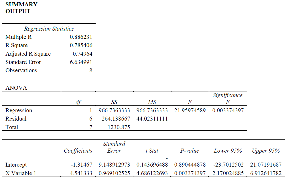
Interpretation of Regression Output

The objective here is to estimate the impact of advertising on sales of the company. First, the model will be specified and the correct or a priori expectation determined. Secondly, the coefficients will be interpreter. Thirdly, the validity of the model will be tested using the following indicators: the coefficient of determination (The R²); the correlation coefficient (r); the t-statistic; p-value and the F-statistic.

The R² which is known as the coefficient of determination shows what proportion of the changes in the dependent variable (sales volume) resulted from changes in the independent variable (advertising expenditures). The R² = 0.78 which means that 78 percent of the changes in the dependent variable were caused by the independent variable. The R² provides a measure of how well future outcomes are likely to be predicted by the model.

Correlation coefficient (r) measures the degree to which two variables vary together or oppositely. The r here is 0.88 which is relatively high and this indicates that advertising (x) and sales (y) are highly positively correlated. The r is also the square root of the R². In the scatter graphs below, when r = +1, both variables are highly positively related; data points will be positively trending. When r = -1, both variables are highly negatively related; data points will be negatively trending.

Another very important statistic to view is that of the actual t-statistic on the regression output,

"$ t = \dfrac{\hat \mu - \mu}{\frac{\hat \sigma}{\sqrt{N}}} $"

 The t-statistic gives a measure of the strength of the coefficient (s). It is the relationship between the coefficient and its standard errors. The lower are the standard errors which is the denominator, the higher will be the t-statistic and the greater will be the strength of the coefficient. On the other hand, the larger are the standard errors relative to the coefficient for that independent variable, the smaller will be the t-statistic and the weaker will be the strength of the coefficient in measuring the impact of the independent variable on the dependent variable. In the output, the t-statistic is 4.68 which is highly significant.

The t-statistic can also be interpreted by doing a hypothesis test. The null hypothesis will indicate that there is no relationship between the dependent variable (sales) and the independent variable (advertising) while the alternative hypothesis will indicate that there is strong relationship between advertising and sales.

H₀ : μ = 0  there is no relationship between advertising and sales

H₁ : μ > 0  there is a very strong relationship between advertising and sales

We will set the level of significance at 5 percent and seek to find the critical value (CV)

The CV is determined from the t-tables by looking in the first column for degrees of freedom (n-1-k) – k is the number of variables – in the question k = 1. In our example, df = 8-1-1= 6. So we will go across to the .05 and down to 6 to get the CV which is 1.94.

We will then compare the t-statistic (4.68) with the CV of 1.94. Because the t-statistic is larger than the CV, we will reject the null hypothesis and accept the alternative hypothesis and conclude that advertising has a significant impact on sales.

We then look at each p-value and see if it is smaller than the 0.5 or 5 percent level of significance. Once the t-statistic is in the rejection region which means that when it is greater than the CV, then the p-value will be less than the level of significance (5 percent or 0.05) and therefore, the null hypothesis can be rejected and the alternative hypothesis can be accepted indicating or confirming that the coefficient has a significant impact on the dependent variable. The p-value is .0033 which is less than the 5 percent level of significance and so the null hypothesis of no relationship between advertising and sales can be rejected.

Regarding the F-statistic, if p = 2, n = 8 then the degrees of freedom will be 2 and 5 producing a CV of 5.79. Because the f Statistic in the output is 21.96 which is larger than the CV of 5.79, we can reject the null hypothesis of no relationship as a package between advertising and sales. Therefore, there is a strong relationship between advertising and sales.

Confidence interval – look at the bottom left of the output and you will see lower 95% and upper 95%. This means the interval between lower 95% and upper 95%. For example, for the independent variable, the coefficient of 4.54 falls in the lower and higher 95 percent; 2.170024885: 6.912641782.

Next - Principles of Business