Previous - Geometry 3: Coordinate Geometry

Frequency Tables

Frequency tables are tables which list the frequency of an event, that is, the number of times an event occurs. There are two types of frequency tables, ungrouped and grouped frequency tables.

Ungrouped

These are frequency tables which list the frequency of observations or data that are ungrouped.

Example: The table below shows the frequency an event occurred.

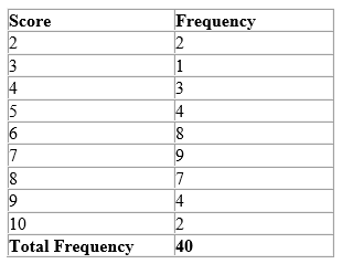
Note:

(1) The total frequency was obtained by summing the frequencies of all the scores.

Grouped

These are frequency tables which list the frequency (number of times) of observations or data that are grouped. These groups are often called classes.

Example:

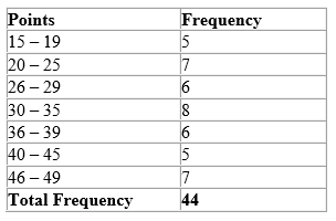
Below is a list of the points each netball team scored in the first half of all 42 games.  This frequency table was constructed for the classes or groups: 15-19, 20-25, 26-29, 30-35, 36-39, 40-45, and 46-49.

Class Limits, Boundaries and Intervals

Class Limits

Class limits are the smallest and largest observations in each class. Therefore, each class has two limits: a lower and upper.

Example:

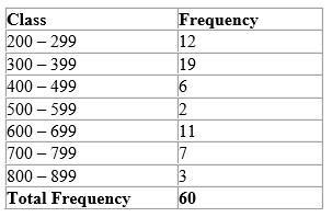
Using the frequency table above, state the lower and upper class limits for the first two classes.

For the first class, 200 – 299

The lower class limit is 200

The upper class limit is 299

For the second class, 300 – 399

The lower class limit is 300

The upper class limit is 399

Class Boundaries

Class Boundaries are the midpoints between the upper class limit of a class and the lower class limit of the next class in the sequence. Therefore, each class has an upper and lower class boundary.

Example:

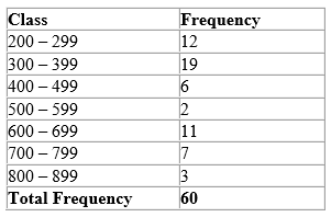
Using the frequency table above, determine the class boundaries of the first three classes.

For the first class, 200 – 299

The lower class boundary is the midpoint between 199 and 200, that is 199.5

The upper class boundary is the midpoint between 299 and 300, that is 299.5

For the second class, 300 – 399

The lower class boundary is the midpoint between 299 and 300, that is 299.5

The upper class boundary is the midpoint between 399 and 400, that is 399.5

For the third class, 400 – 499

The lower class boundary is the midpoint between 399 and 400, that is 399.5

The upper class boundary is the midpoint between 499 and 500, that is 499.5

Class Intervals

Class interval is the difference between the upper and lower class boundaries of any class.

Example:

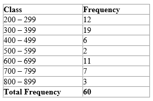
Using the table above, determine the class intervals for the first class.

For the first class, 200 – 299

The class interval = Upper class boundary – lower class boundary

Upper class boundary = 299.5

Lower class boundary = 199.5

Therefore, the class interval = 299.5 – 199.5

= 100

Mean

The mean of a given set of numbers is the average of those numbers, and is calculated by summing all the numbers and dividing by the amount of numbers.

That is, the mean  = (the sum of the numbers)/the amount of numbers

Example:

Find the mean of the following numbers:

4, 5, 6, 12, 15, 20

(4+ 5 + 6 + 12 + 15 + 20)/6 = 10.3

The above is for the case of ungroup data.  To find the mean of a frequency distribution with grouped data, the product of the frequency and the corresponding observations is calculated and summed.  That result is then divided by the sum of the frequency amounts.

That is, the mean

=Ʃfx

where,  Ʃfx is the sum of the products of the frequency and the corresponding observations

and Ʃf is the sum of the frequencies.

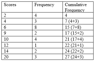
Example:

The table below shows the sizes of an item based on a survey of 50 boys.

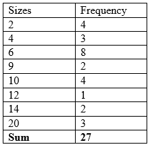
Find the mean score.

Rule to find the mean:

• Multiply the frequencies by the corresponding observations.
• Sum the product of the frequencies and the observations.
• Sum the frequencies.
• Divide the sum of the products of the frequencies and observations by the sum of the frequencies.

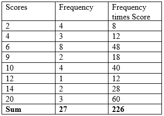
Therefore, Ʃfx = 226

And,            Ʃf = 27

That is, the mean

226/27 = 8.4

Furthermore, to find the mean of a frequency distribution with grouped data, we can find the mid-point of each class interval, then find the product of the frequency and the corresponding mid-points (noted as f₁ x₁) and sum them, that sum is then divided by the sum of the frequency amounts.

Example:

Find the mean of the following data.

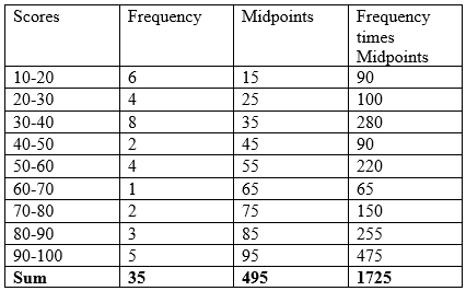
Procedure to find the mean:

• Find the mid-point of each class by adding the lower class limit and the upper class limit of each class, and dividing by two.
• Multiply the mid-points of each class by the respective frequencies.
• Sum the product of the mid-points and the frequencies.
• Sum the frequencies.
• Divide the sum of the products of the mid-points and the frequencies by the sum of the frequencies.

Therefore, Ʃf₁ x₁ = 1725

And Ʃf₁ = 35

That is, the mean

1725/35 = 49.3

Cumulative Frequency

The cumulative frequency is obtained by adding each frequency in the table, to the cumulative frequency in the row above it.

Example:

Insert a cumulative frequency column into the table below.

Median

The median of a given set of numbers or ungrouped data is the central number (the number in the middle). To find the median, the set of numbers should either be arranged in ascending (smallest to largest) or descending (largest to smallest) order. If there is an odd amount of numbers in the set, then the median is the middle or central number.  If there is an even amount of numbers in a set, then the median is the average of the two central numbers

Example:

Find the median of the following set of numbers.

322, 330, 328, 323, 326, 324, 327, 325, 329

Solution

The numbers in ascending order:

322, 323, 324, 325, 326, 327, 328, 329, 330

The central number is, 326 and therefore the median is 326.  This is so because the amount of numbers is odd.

Example:

3, 4, 4, 4, 5, 5, 5, 6, 7, 8

Solution

Since the number of observations (n) is even then we take the average of the two middle or central numbers which is:

(5 + 5)/2 = 5.

Alternatively, to find the median of ungrouped data, if the sum of the frequency (n) is an odd number, then the median is the observation, if the sum of the frequency (n) is an even number, then the median is the average of  and  observations.

Taking the above example of:

3, 4, 4, 4, 5, 5, 5, 6, 7, 8,

the median = 10/2 = 5 and 10/2 + 1 = 6 or the 5^th and 6^th numbers which are 5 and 5.  So the median is the average of these two numbers which is 5+5=10/2 = 5.  Note that this is the same answer as when simply taking the average of the two middle numbers. 

Example:

Find the median of the data below.

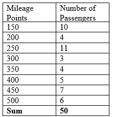
The number of observations (employees), (n) = 50

Since 50 is an even number, the median is the average of the  and  observations.

That is, the average of

50^th/2 and (50/2 + 1)^th observations

25^th and 26^th

The next step is to insert a cumulative frequency column.

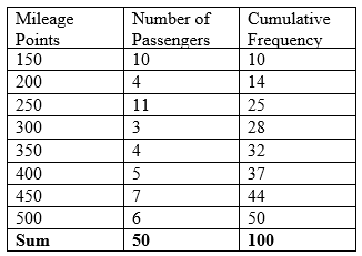
Identify which row 25 falls under in the cumulative frequency column that corresponds to the mileage points in that row of the 25^th observation.  That is, the 25^th observation is 250.

Identify which row 26 falls under in the cumulative frequency column that corresponds to the mileage points in that row of the 26^th observation.  That is, the 26^th observation is 300.

Therefore, the median

(300 + 250)/2

= 275

Therefore, the medial is 275.

Mode

The mode of a given set of numbers is the number which has the highest frequency, that is, it is listed the most times.

Example:

The mode in the following distributions

(i) 5, 12, 14, 12, 26, 12, 12, 24

is 12 because it appears the most times.

(ii) Find the mode for the following data.

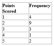
The highest frequency is 9.

Therefore the modal number of goals scored is 2.

Range, Interquartile and Semi-interquartile Ranges (Raw Data)

Range

The range of a set of numbers is the difference between the largest and the smallest number.

Example:

Calculate the range of the following numbers:

322, 323, 324. 325, 326, 327, 328, 329, 330.

The range

= the largest number – the smallest number

=  330 – 322

=  8

The range of a frequency distribution with ungrouped events is calculated using the formula:

Range = the upper boundary limit of the largest event – the lower boundary limit of the smallest event

Example:

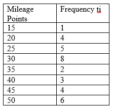
Find the range of the points in the following table

Firstly identify the largest and smallest points.

Largest point = 50

Smallest point = 15

Find the upper boundary limit of the largest and the lower boundary limit of the smallest.

Upper boundary limit of 50 is, 50.5

Lower boundary limit of 15 is, 14.5

The range = Upper boundary limit of 50 – lower boundary limit of 15

= 50.5 – 14.5

= 36

Quartiles

• Q₂ (the middle quartile) is the median.
• Q₁ (the lower quartile) is the median of the numbers to the left of, or below Q₂.
• Q₃ (the upper quartile) is the median of the numbers to the right of, or above Q₂.

Example:

12, 14, 16, 18, 20, 22, 24, 26, 28, 30, 32, 36, 38, 40, 42

Find the lower, middle and upper quartiles of the data above.

Since the data is already in ascending order, identify the median.

12, 14, 16, 18, 20, 22, 24, 26, 28, 30, 32, 36, 38, 40, 42

26 is the median, therefore, Q₂= 26

The median of the numbers to the left of Q₂: 12, 14, 16, 18, 20, 22, 24

18 is the median, therefore, Q₁ = 18

The median of the numbers to the right of Q₂: 28, 30, 32, 36, 38, 40, 42

36 is the median, therefore, Q₃ = 36

Interquartile Range

The interquartile range of a distribution is the difference between the upper and lower quartiles.

That is, interquartile range = Q₃ – Q₁

Therefore using the example above, the interquartile range is:

Interquartile range = Q₃ – Q₁

Since,

Q₃ = 36

Q₁ = 18

Interquartile range is therefore

= 36 – 18

= 18

Semi-Interquartile Range

The semi-interquartile range of a distribution is half the difference between the upper and lower quartiles, or half the interquartile range.

Therefore, from the example above, it was determined that the interquartile range = 18.

Therefore, semi-interquartile range = 18/2 = 9.

Probability

Probability is defined as the likelihood of an event occurring. Given that all the possible outcomes are equally likely, the probability of an event is equal to the number of favourable outcomes divided by the total number of possible outcomes, that is:

Probability of an event = number of favourable outcomes/total number of possible outcomes

The probability of an event will be a number between 0 and 1. If the probability of an event is 0, this means that the event will never occur and if the probability of an event is 1, this means that  the event will occur.

Example:

A basket contains 20 marbles. There are 4 red marbles, 5 blue marbles, 1 yellow marble and 10 green marbles. 

1. What is the probability of selecting a red marble?
2. What is the probability of selecting a blue marble?
3. What is the probability of selecting a yellow marble?
4. What is the probability of selecting a green marble?

Rules:

• Determine the number of favourable outcomes.
• Determine the total number of possible outcomes.
• Divide the number of favourable outcomes by the total number of possible outcomes.

1. The number of favourable outcomes = the number of red marbles is 4. The total number of possible outcomes = the number of marbles in the basket is 20. Therefore, the probability of choosing a red marble is 4/20 = 1/5 = 0.2.
2. The number of favourable outcomes = the number of blue marbles is 5. The total number of possible outcomes = the number of marbles in the basket is 20. Therefore, the probability of choosing a blue marble is 5/20 = 1/4 = 0.25.
3. The number of favourable outcomes = the number of yellow marbles is 1. The total number of possible outcomes = the number of marbles in the basket is 20. Therefore, the probability of choosing a yellow marble is 1/20 = 0.05.
4. The number of favourable outcomes = the number of green marbles is 10. The total number of possible outcomes = the number of marbles in the basket is 20. Therefore, the probability of choosing a green marble is 10/20 = 1/2 = 0.5.

Next - Consumer Arithmetic