Central tendency is what is known as the centre or central position of a data set. There are three measures of central tendency which are: mean, median and mode. The mean is simply the average.
Mean
The arithmetic mean of a set of observations is the total sum of the observations divided by the number of observations.
Find the mean monthly rainfall in a particular area using the following data.
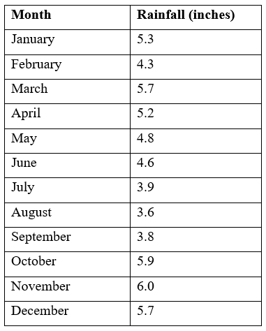
We will use the sigma notation to work out this problem. We let the variable x denote the rainfall in Town A in each month. Then "$ \sum x $" represents the total rainfall for the given year. Remembering that there are 12 months in the year, we can calculate the mean monthly rainfall in inches (denoted by the symbol x ) as:
"$ \bbox[5px,border:2px solid black] { \bar x = \frac {\sum x}{n} } $"
where :
"$ \bar x $" represents the arithmetic mean of the sample of observations;
"$ x $" represents the sample of observations;
"$ \sum x $" represents the sum of the sample of observations;
"$ n $" represents the number of observations.
"$ Mean = 58.8/12 = 4.9$".
Group Mean
The following table shows the frequency distribution of the number of days on which 100 employees of a firm were late for work in a given month. Using this data, find the mean number of days on which an employee is late in a month.
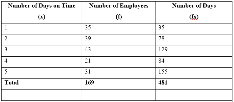
Let "$x = $" the possible values for the number of days late
"$f =$" the frequencies associated with each possible value of "$x$"
Then:
Total number of days on time = "$ \sum fx = 481 $"
Total number of employees = "$169$"
and,
"$ Mean = \sum fx / \sum f = 481/169= 2.85$"
Example:
You are given a frequency distribution of class boundaries shown in the following Table. As in the above Example, the data are grouped into a number of classes, but the variable, x, is a measurement, so it is continuous and it is quite likely that all the 85 values are different. The frequency distribution only tells us the class boundaries, e.g. we know that 7 observations lie between 160 and 165 cm but we do not know any of their values. To calculate the mean we must have a single value of x which is typical of all the values in each class. We choose the midpoint of each class as this typical value and assume that each observation in the class is equal to the midpoint value.
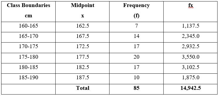
Let "$x = $" the midpoints of the classes
"$ f = $" frequencies associated with each class
"$ Mean = 14,842.5/85 = 175.79 $"
Median
On arranging the data in ascending or descending order median is the middle – most observation. If the number of observations are odd then the median is "$ (n+1 / 2) th $" observation where "$ 'n' $" is the number of observations. If number of observations are even then median is the average of "$ (n / 2) th $" and "$( n / 2 + 1) th $" observation.
"$ 36; 3.8; 3.9; 4.3; 4.6; 4.8; 5.2; 5.3; 5.7; 5.7; 5.9; 6.0 $"
The median of the above dataset is the mean of the "$6^{th}$" and "$ 7^{th} $" numbers which is:
"$(4.8 + 5.2)/2 = 5$".
Median of Grouped Data
Having learnt to calculate the individual median, we turn to calculate the median for group data.
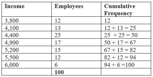
Here, the number of observations "$(n) = 100$". This is an even number, so the median is average of "$( n / 2 )th $" and "$(n / 2 + 1)th $" observations i.e. average of "$( 100 / 2 )th$" and "$ [(100 / 2) + 1]th $" observation. i.e. average of "$50th$" and "$51th$" observations. To find these observations let us arrange the data in the following manner.
So, the "$50th$" observation is "$4400$" and "$51th$" observation is "$4900$".
"$ \text{Median} = (4400 + 4900) / 2 $"
"$ \text{Median} = 9300 / 2 $"
"$ \text{Median} = 4650 $".
This means 50% workers got wages less than 4650 and another 50% got more than 4650.
Example: from the following table, find the median mark for students in a class.
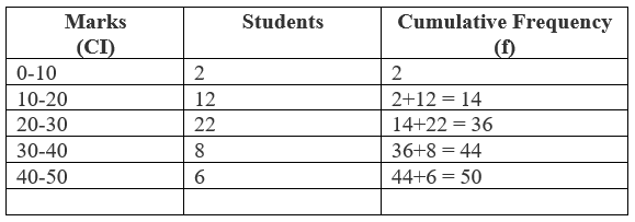
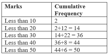
First, we calculate n / 2, with its help we determine the class whose cumulative frequency is nearly equal to n /2. This class is known as median class. Then, the median is calculated by the following formula:
"$ \text{Median} = L + \begin{pmatrix} n/2 - \text {cf} \\ \hline \text{f} \end{pmatrix} \times n $"
"$ \text{Median} = $"
"$ L = $" lower limit of median class
"$ \text {cf} = $" cumulative frequency of class prior to median class.
"$ \text{f} = $" frequency of median class.
"$ n = $" class size.
Here "$ n / 2 = 50 / 2 = 25 $"
So, "$ 20 -30$" is the median class.
Now, "$ L = 20 $"
"$ n = 10 $"
"$ cf = 14 $"
"$ f = 22 $"
Using
"$ \text{Median} = L + \begin{pmatrix} n/2 - \text {cf} \\ \hline \text{f} \end{pmatrix} \times n $"
"$ Median = 20 + [(25 - 14) / 22] x 10 $"
"$ Median = 20 + (11 / 22) x 10 $"
"$ Median = 20 + 5 $"
"$ Median = 25 $".
This means 50% of the students got less than 25 marks and other 50% got more than 25 marks.
Mode
The mode of given data is the observation which is repeated maximum number time. For example, in the following case, the mode will be 50 because it is that number that occurred more frequently: 32, 50, 35, 50, 33, 50, 42, 50, 50. Find the mode of the above data.
Mode of Grouped Data
You have seen that by just observing the given ungrouped data carefully its mode can be obtained. However, for grouped data it is not possible to find the mode just by observation. This can be obtained using the following formula:
"$ \text{Mode} = L + \begin{pmatrix} \text {f}_1 - \text {f}_0 \\ \hline \text{2f}_1 – \text{f}_0 – \text{f}_2 \end{pmatrix} \times n $"
Here,
"$ L = $" lower limit of modal class
"$ \text{f}_1 = $" frequency of modal class
"$ \text{f}_0 = $" frequency of class preceding the modal class.
"$ \text{f}_2 = $" frequency of class succeeding the modal class.
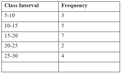
Here frequency of class interval 15 - 20 is maximum.
So, it is the modal class
Now
"$L =$" the lower limit of modal class = 15
"$ \text{f}_1 =$" frequency of modal class = 7
"$ \text{f}_0 =$" frequency of class preceding the modal class = 5
"$ \text{f}_2 =$" frequency of class succeeding the modal class = 2
"$h =$" size of class intervals = 5
So,
Using, "$ \text{Mode} = L + \begin{pmatrix} \text {f}_1 - \text {f}_0 \\ \hline \text{2f}_1 – \text{f}_0 – \text{f}_2 \end{pmatrix} \times h $"
We have,
"$Mode = 15 + [(7 - 5) / (2 x 7 - 5 - 2)] \times 5 $"
"$Mode = 15 + [2 / (14 - 7)] \times 5 $"
"$Mode = 15 + (2 / 7) \times 5 $"
"$Mode = 15 + (10 / 7) $"
"$Mode = 15 + 1.42 $"
"$Mode = 16.42 $".