The Macroeconomic Model
A macroeconomic model is an analytical tool designed to describe the operation of the economy of a country. These models are usually designed to examine the dynamics of aggregate quantities such as the total amount of goods and services produced, total income earned, the level of employment of productive resources and the level of prices.
The Closed Economy
In building the macroeconomic model, the following are some key assumptions:
- The price level will be held constant and will not vary with the level of income.
- The economy is operating at full capacity.
- There is no trade and so the economy is closed to the world; so we will have only consumers ( C) and firms (I);
- There is no government sector as yet.
We call such an economy a closed or two-sector economy where there is no G and X-M in the model. In such an economy, GDP will be measured or represented by:
GDP = AD = C + I
where
C – consumption,
I – investments.
To proceed in building the income model for the two-sector economy (C+I), we know that parts of income are spent and other parts are saved and the determination of these are through the consumption and savings functions.
The Consumption Function
The consumption function describes the relationship between disposable income and consumption.
C = a0 + b1 Y
where:
C = consumer spending,
a0 = autonomous consumption, or the level of consumption that would still exist even if income was $0
b1 = marginal propensity to consume which is the change in consumption as a result of 1-unit change in disposable income
Y = real disposable income
The Savings Function
What is not consumed is saved and is shown as the savings function which is as follows
S = a0 + b1 Y
S = saving;
a0 = autonomous saving or the level of savings that would still exist even if income was $0
b1 = marginal propensity to save, which is the change in savings as a result of 1-unit change in disposable income
The Three-Sector Economy
In the preceding discussion, the case was for the two-sector economy. When we add the government sector we will now transform the two-sector economy to a three-sector economy where AD = AE = Y = C + I + G. Notice that when we add the governments sector, aggregate income increases and so the aggregate income or demand curve moves up above the two-sector AD curve. Now with the government sector added, we also have taxes which are like a leakage from the circular flow of income. Also notice that equilibrium will now be,
AD = C + I + G = C + S + T, where injections equal to leakages.
Open Economy
The model of the closed economy was constructed above where it was assumed that there is no trade meaning no exports and imports. This was only for purposes of simplicity. Now we will introduce both trade and government sectors and this will transform the two-sector model of AD = AE = C + I into the four-sector or open economy as:
AD = AE = C + I + G + X – M
The addition of the government and trade sectors will shift the aggregate expenditures curve upwards as seen in the following graph.
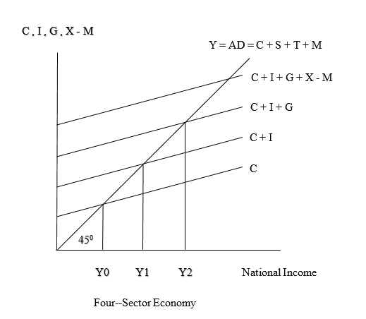
We can see that when the trade sector is added, aggregate demand and supply increase and so the AD curves moves up from C + I to C + I + G then to C + I + G + X - M
The Multiplier Effect
When variables such as I or C change, GDP will change by a larger amount than the change in I or C. This is called the multiplier effect. For example, assume that there is a project which involves the construction of a factory that will cost $100.00 million. Workers in this industry will earn income that they will spend on other things. This will cause an increase in real GDP. With this new level of GDP, more incomes will be earned and spent which will cause further increases in incomes and GDP. Therefore the initial increase in spending of $100.0 million would have resulted in an increase in GDP by much more than the initial $100.0 million. This is what is referred to as the multiplier effect. The multiplier can be represented as:
"$ K = \Delta Y / \Delta I $", the change in GDP resulting from the change in investment.
There are two types of multipliers which are the spending multiplier and the multiplier effect.
Example:
To illustrate this, let us take a look at a very simple economy comprising of four companies:
- Shannon who is the store owner;
- Derrick who works on an assembly line in a car factory;
- Joe who is a food mart owner and;
- Davis who owns a hardware store.
Derrick’s factory has a profitable year and so earns an extra $1,000 of income. Derrick decided to spend $800 on clothes. Since Shannon is a store owner, Derrick spends this $800 at Shannon’s store so then Shannon will earn $800. Shannon also decides to spend part of this $800 she receives which is $600 on things that she desires. She spent this on Joe’s food mart. This is additional income for Joe who then goes to Davis and spends $500 on tools. As we can see, the initial $1,000 spending leads to three more rounds of spending with smaller amounts each time. Total spending was $1,000 + $800 + $600 + $500 = $2,900. When money spent multiplies in this manner, we refer to it as the multiplier effect. Money spent in the economy does not stop with the first transaction.
In the above case we know that income increased by a multiple of the initial spending. This was referred to as the multiplier effect. However, we did not know by how much but we can know by the following formula:
"$ \text{Spending multiplier} = \frac{1}{MPS} = \frac{1}{1 − MPC} $"
where,
MPS stands for marginal propensity to save which is the percentage of any increase in income which households are going to save; and MPC stands for marginal propensity to consume and it is the percentage of any increase in income which households are expected to consume.
By definition, MPS + MPC = 1 and MPS = 1 − MPC.
This is known as the spending multiplier which can be differentiated from the multiplier effect. As an example, suppose a large factory is to be built which will cost $8 million. This $8 million which is spent to build the factory will go as income to the workers who are constructing factory. When this $8 million is spent by the workers to buy goods and services, it will multiply throughout the economy. The final amount the $8 million will multiply to can be determined if we know the marginal propensity to consume which in this case is 0.8. Using the above multiplier formula of:
"$ \frac{1}{1 – MPS} = \frac{1}{MPC} $"
= 1/(1-0.8) = 1/0.2 which is = 5
When we multiply this 5 by the initial amount spent to construct the factory which is $8 million, this $8 million will multiply to $40 million ($8 multiply by 5). It is important to note that higher consumption will lead to a higher multiple.