What Is Consumer Theory
Consumer theory is the study of how consumers make decisions regarding how to spend their money on goods and services given their preferences and their budget constraints. Consumer theory shows how individuals make choices given their income and the prices of goods and services. There are two main theories of consumer choice which are the ordinalist or indifference curve approach and the cardinalist or marginal utility approach.
The Ordinalist or Indifference Curve Approach
The ordinalist or indifference curve approach to consumer theory requires the use of indifference curves and the budget constraints. An indifference curve is a graph that shows combinations of goods that give the consumer equal satisfaction or utility. That is, at each point on the curve, the consumer has no preference for one bundle or combination of goods over another. In other words, they are all equally preferred.
The indifference curve is combined with the budget line (which shows the budget constraint) to produce the optimum position of the consumer. The budget line shows the combination of goods that can be afforded with the current level of income.
In fact, where the indifference curve is tangent to the budget line constitutes the optimum position which is where the arrow is pointing at A in the following graph. Points under this point are attainable but will not result in the consumer maximizing his utility. Points above this optimum point cannot be attained because the consumer cannot afford such combinations of goods with his or her existing income. The consumer is constrained by the budget line which represents his maximum income. The budget line is derived as follows: If income is $10.00 and there are two products for consumption (x and y), and if the price of x is $1.00 and the price of y is $2.00, when the consumer chooses to consume all of x and none of y, his point will be 10 units on the vertical axis. When the consumer consumes all of y and none of x, the budget constraint will be at 5 on the horizontal axis as can be seen in the following graph.
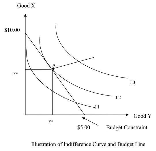
In order for the consumer to consume more of Y he must consume less of X. This is the change in Y divided by the change in X which is the marginal rate of substitution. As we move down the indifference curve, the slope decreases because more and more of Y will require less and less of X. This is what is referred to as diminishing marginal utility. We can also find the slope of the budget line from the equation of the budget line as is stated below:
"$BL = Px \cdot X + Py \cdot Y$"
"$ \Delta Y / \Delta X = - P_x / P_y $"
"$ P_x / P_y $" is the opportunity cost of X in terms of Y.
Hicksian Substitution and Income Effects of Price Change
Income Effect and a Substitution Effect
Every price change can be converted into an income effect and a substitution effect. The substitution effect is basically a price change that changes the slope of the budget constraint, but leaves the consumer on the same indifference curve. This effect will always cause the consumer to substitute away from the good that is becoming comparatively more expensive. The substitution effect can be separated from the income effect using two approaches: the Hicksian and the Slutsky approaches.
To illustrate the Hicksian approach (named after J R Hicks), we have two goods which are X and Y. Assume that the price of Good Y falls from $2.00 to $1.00. The budget line will shift from BC1 to BC2 – the consumer will be able to purchase more of Good Y. Resulting from this price fall of Good Y is a new indifference curve I2 and a new equilibrium point B. As a result of this price decline, quantity demanded of Good Y increases from Y1 to Y2 as can be seen in the following graph. This represents the total effect of the price change which is the substitution effect plus the income effect.
The substitution effect is the change in consumption pattern of a good due to a change in the relative prices of goods. The income effect is the change in consumption patterns due to the change in purchasing power or real income when the price of one product falls while the price of other products and nominal income remain unchanged.
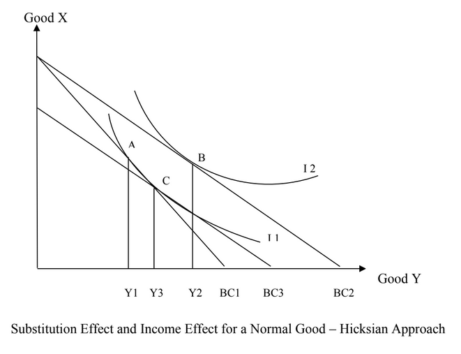
Now we need to separate these two effects. In order to do so, we need to keep the real income constant i.e., eliminating the income effect to calculate substitution effect. According to the Hicksian method of eliminating income effect, we just reduce consumer’s money income so that the consumer remains on his original indifference curve "$IC_1$" , keeping in view the fall in the price of commodity Y. A reduction in consumer’s money income is done by drawing an imaginary budget line BC3. At the same time, the new parallel price line BC3 is tangent to the original indifference curve "$IC_1$" at point C. Hence, the consumer’s equilibrium changes from point A to point C. This means that an increase in quantity demanded of Good Y from Y1 to Y3 is purely because of the substitution effect. Therefore, the reason for drawing the imaginary line is to keep the consumer on his same level of income because the fall in the price of Good Y caused an increase in real income. In this case, the substitution effect from the fall in the price of Good Y is from A to C or from Y1 to Y3 and the income effect is from C to B or from Y3 to Y2.
Marginal Utility or Cardinalist Approach
Total utility refers to the total satisfaction that a customer receives from all units of a product consumed. Marginal utility refers to the change in satisfaction that the customer receives from consuming one more or less unit of that product. An important aspect of the marginal utility approach is that of the law of diminishing marginal utility. The law of diminishing marginal utility states that when more and more of a product is being consumed, the consumer will be getting less and less satisfaction from the consumption of that good holding all other things constant.
In marginal utility theory, the analysis can be conceptualized by obtaining the marginal utility to price ratio such as follows:
"$ MU_x / P_x $"
where
"$ MU_x $" = marginal utility of product X and,
"$ P_x $" = is the price of X
This ratio states the extra utility or satisfaction that a consumer gets from every dollar spent on this good which is Good X in this case. For example, if Good X costs $5, and the marginal utility of consuming 5 units of Product X is 20, then the "$ MU_x / P_x $" , will be: "$ 20 / 5 = 4 $" utils per dollar.
As a rule using the marginal utility approach, in order to maximize utility, the consumer must allocate his expenditures so that the marginal utility per dollar spent on Good X is equal to the marginal utility per dollar spent on Good Y. This can be stated as:
"$ MU_x / P_x = MU_y / P_y $"
where
"$ MU_x$" = marginal utility of Good X and,
"$P_x$" = is the price of Good X
"$MU_y$" = marginal utility of Good Y and,
"$P_y$" = is the price of Good Y.