Previous - Discrete Random Variables And Their Probability Distribution

Continuous Probability Distribution – Normal Distribution

A continuous random variable is one that cannot be counted but rather is estimated to be in a range or interval. The normal distribution is one of the many probability distributions that a continuous random variable can possess. A large number of phenomena in the real world are normally distributed.

The properties of a normal probability distribution:

1. the total area under the curve is 1.0;
2. the curve is symmetric about the mean – the mean is in the middle and;
3. the two tails of the curve extend indefinitely.

The mean μ and the standard deviation σ are the parameters of the normal curve. Given the values of these two variables, we can find the area under the normal distribution curve for any interval. The value of μ determines the centre of the normal distribution curve on the horizontal axis and the value of σ gives the spread of the normal distribution curve.

Standard Normal Distribution

The standard normal distribution is a specific case of the normal distribution. For the standard normal distribution, the value of the mean is zero and the value of the standard deviation is equal to 1. The random variable that possesses the standard normal distribution is denoted by z; in other words, the units for the standard normal distribution are denoted by z and are called z scores or z values. The horizontal axis is labeled z.

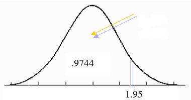
The z values at the right of the mean are positive and those to the left are negative. The z-value for a point on the horizontal axis gives the distance between the mean and that point in terms of the standard deviation. As an example, a z-score of 2 is two standard deviations to the right of the mean and a z score of minus 2 is two standard deviations to the left of the mean. If we want to find the area under the curve with a z score of 1.95, we simply look in the z-table. We look at 1.9 in the left column and look for the .05 at the top of the table. The area under the curve corresponding to a score is .9744.

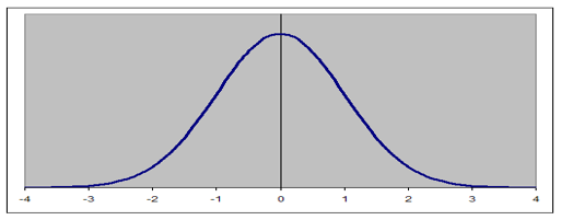
When the population and sample are normally distributed, the normal distribution curve will be as below,

Example 1:

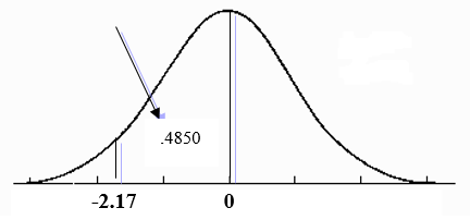
Find the area under the normal curve from z = -2.17 to z=0.

Solution:

This will require that we find the areas to the left of 0 and to the left of -2.17.  The area to the left of 0 is .5000 and the area to the left of -2.17 is .0150.  We therefore take the difference which is "$ .5000-.0150 = .4850 $".   Therefore, the area from 0 to -2.17 is
"$ P(-2.17 \leq z \leq 0) = .5000 - .0150 = .4850 $"

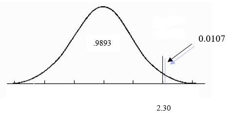
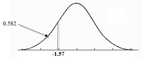
Example2:

Find the following areas under the standard normal curve:

1. area to the right of z = 2.30 and;
2. area to the left of z = -1.57.

Solution:

1. The normal distribution table gives the area to the left of a z value. Therefore, in order to find the area to the right of 2.30, we will need to find the area to the left of 2.30 and minus it from the total area under the curve which is 1.0.

   "$ P(z \leq 2.30) = 1.0 - .9893 = .0107 $"

   

2. The area to the left of -1.57 is the z score for that value. It is "$P(z \lt -1.57) = .0582$".

   

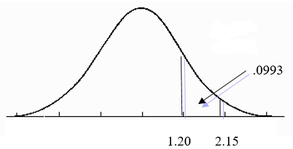
Example 3:

Find the probabilities for the following standard normal curve:

1. "$ P \left( 1.20 \lt z \lt 15 \right) $"
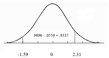
2. "$ \left(-1.59 \lt z \lt 31 \right) $"

Solution:

1. We will need to obtain the area: to the left of 1.20 which is .8849 and;
   to the left of 2.15 = .9842.

   Therefore, the area between 1.20 and 2.15 is .9842 - .8849 = .0993.

   

Solution:

2. To find the area between -1.56 and 2.31, we do as above. We find the area to the left of -1.59 which is .0559 and to the left of 2.31 which is .9896. We then take the difference which is  .9896 - .0559 = .9337.

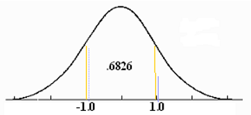
1. The total area within 1 standard deviation of the mean is .6828 or 68.26 percent.

   "$ P \left(-1.0 \leq z \leq 1.0 \right) = .8413 - .1587 = .6826 $"

   "$ P \left(\mu - 1 \sigma \leq x \leq \mu +1 \sigma \right) = .8413 - .1587 = .6826 $"

   

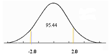
2. The total area within 2 standard deviations of the mean is .9544 or 95.44 percent.

   "$ P \left(-2.0 \leq z \leq 2.0 \right) = .9772 - .0228 = .9544 \text { or } 95.44 \text { percent} $"

   "$ P \left( \mu - 1 \sigma \leq x \leq \mu +1 \sigma \right) = .9772 - .0228 = .9544 \text { or } 95.44 \text { percent} $"

   

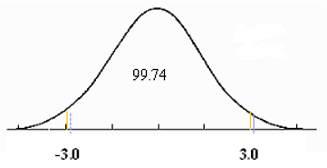
3. the total area within 3 standard deviations of the mean is .9974 or 99.74 percent.

   "$P \left( -3.0 \leq z \leq 3.0 \right) = .9987 - .0013 = .9974 \text { or } 99.74 \text{ percent } $"

   

Standardizing a Normal Distribution

As was seen earlier, the z-scores can be used to find areas under the normal curve.  However, there are times when the random variable may have a normal distribution where the values of the mean and standard deviation are different from 0 and 1 respectively.  The first step in the solution of this matter is to convert the normal distribution to a standard normal distribution. This procedure is called standardizing the normal distribution.  For a normal random variable x, a particular value of x can be converted to its corresponding z value by using the following formula:

"$ Z = \dfrac{x - \mu}{\sigma} $"

where, "$ \mu $" and "$ \sigma $" are the mean and standard deviation of x.

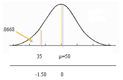
Example 4:

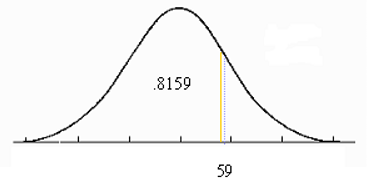
Let x be a continuous random variable that has a normal distribution and a mean of 50 and a standard deviation of 10.  Convert the following x values to z values and find the probabilities to the left of these points:

1. x = 59 and
2. x = 35

Solution:

1. "$ z = \dfrac{\left( 59-50 \right) }{10} = .90 $"

   We look for .90 in the z table and get .8159. Therefore, the probability of x being to the left of 55 is .8159 or 81.59 percent.

2. "$ z = \dfrac{\left( 35-50 \right) }{10} = -1.50 $".

   so the probability of x being less than 35 is "$ P \left( x \lt 35 \right) = P \left( z \lt 1.50 \right) = .0668 \text{ or } 6.68 \text { percent} $".

   

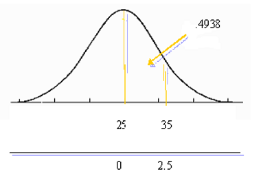
Example 5:

Let x be a continuous random variable that is normally distributed with a mean of 25 and a standard deviation of 4.  Find the area between:

1. x=25 and x=35 and;
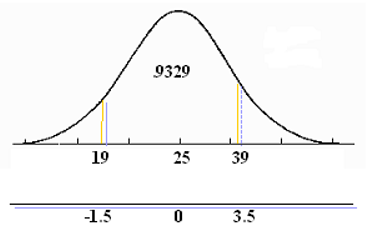
2. x=19 and x=39

Solution:

1. "$ Z = \dfrac{x - \mu}{\sigma} $" 

   "$ Z = \dfrac{ \left( 0-0 \right)}{4} = 0 $"

   "$ Z = \dfrac{ \left( 35-25 \right) }{4} = \dfrac{10}{4} = 2.5 $"

   To obtain the area of x being between 25 and 35, we look for the z values in the table corresponding to these two values: we obtain .5 for x=25 and .9938 for z = 2.5.  Therefore the probability of x being between 25 and 35 is: .9938 - .5 = .4938.

   

2. "$ z = \dfrac{ \left( 19-25 \right) }{4} = -1.5 $"

   "$ z = \dfrac{\left( 39-25 \right)}{4} = 3.5 $"

   Hence, the required area between x being between 19 and 35 is: "$ P \left( 19 \lt x \lt 35 \right) = P \left( z-1.5 \lt z \lt 3.5 \right) = .9997 - .0668 = .9329 $" or the probability of x being between 19 and 39 is 93.29 percent.

   

Example 6:

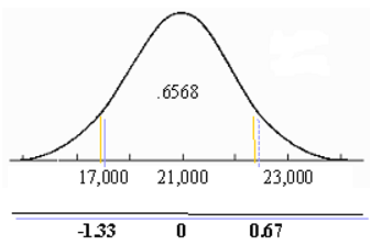
According to an estimate, the average price paid for a motor vehicle in the 2010 in Trinidad and Tobago was $21,000.  Suppose such average price have normal distribution with a mean of $21,000 and a standard deviation of $3,000.  From a random sample of the car buying population, find the probability that such price is between $17,000 and $23,000.

Let x be the consumer debt of a randomly selected Jamaican household.  Then x is normally distributed with:

"$ \mu = $21,000 \text{ and } \sigma = $3,000 $"

Therefore,

"$ \begin{align} z &= \dfrac{ \left( 17,000 - 21,000 \right)}{3,000} \\ &= \frac{-4,000}{3,000} \\ &= -1.33 \end{align} $"

"$ \begin{align} z &= \dfrac{ \left( 23,000 - 21,000 \right)}{3,000} \\ &= \frac{2,000}{3,000} \\ &= 0.67 \end{align} $"

Drawing the normal curve and viewing the z values in the tables, we see that:

-1.33 corresponds to a z value of .0918 and 0.67 corresponds to a z value of .7486.

Therefore,

"$ P \left( $17,000 \lt x \lt $23,000 \right) = P \left( -1.33 \lt z \lt .54 \right) = .7486-.0918 = .6568 $"

Therefore, the probability that the average car price will be between $17,000 and $23,000 is .6568 or 65.68 percent. 

Next - Difference Between Z Distribution And T Distribution